Sea Cucumber Essence

Cross-posted on GitHub. There are also slides from my lightning talk at the Human Aligned AI Summer School 2022.

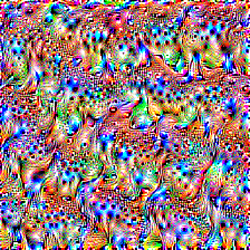
In short, why does this (maximized node 4 in the block5_conv4 layer of VGG19)

node4

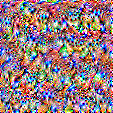
look like sea_cucumber to all ImageNet-trained CNNs?

tSNE

Context

Using my feature extraction script I analyzed node 4 in the block5_conv4 layer of VGG19:

import numpy as np
import matplotlib.pyplot as plt
import tensorflow as tf
from tensorflow.keras.preprocessing import image
from PIL import Image 


base_model = tf.keras.applications.VGG19(include_top=False, weights='imagenet')
target_layer="block5_conv4"
target_index=4
steps=100
step_size=0.1
# Take the network and cut it off at the layer we want to analyze,
# i.e. we only need the part from the input to the target_layer.
target = [base_model.get_layer(target_layer).output]
part_model = tf.keras.Model(inputs=base_model.input, outputs=target)


# The next part is the function to maximize the target layer/node by
# adjusting the input, equivalent to the usual gradient descent but
# gradient ascent. Run an optimization loop:
activation = None
@tf.function(
    # Decorator to increase the speed of the gradient_ascent function
    input_signature=(
        tf.TensorSpec(shape=[None,None,3], dtype=tf.float32),
        tf.TensorSpec(shape=[], dtype=tf.int32),
        tf.TensorSpec(shape=[], dtype=tf.float32),)
)
def gradient_ascent(img, steps, step_size):
    loss = tf.constant(0.0)
    for n in tf.range(steps):
        # As in normal NN training, you want to record the computation
        # of the forward-pass (the part_model call below) to compute the
        # gradient afterwards. This is what tf.GradientTape does.
        with tf.GradientTape() as tape:
            tape.watch(img)
            # Forward-pass (compute the activation given our image)
            activation = part_model(tf.expand_dims(img, axis=0))
            print(activation)
            print(np.shape(activation))
            # The activation will be of shape (1,N,N,L) where N is related to
            # the resolution of the input image (assuming our target layer is
            # a convolutional filter), and L is the size of the layer. E.g. for a
            # 256x256 image in "block4_conv1" of VGG19, this will be
            # (1,32,32,512) -- we select one of the 512 nodes (index) and
            # average over the rest (you can average selectively to affect
            # only part of the image but there's not really a point):
            loss = tf.math.reduce_mean(activation[:,:,:,target_index])

        # Get the gradient, i.e. derivative of "loss" with respect to input
        # and normalize.
        gradients = tape.gradient(loss, img)
        gradients /= tf.math.reduce_std(gradients)

        # In the final step move the image in the direction of the gradient to
# increate the "loss" (our targeted activation). Note that the sign here
# is opposite to the typical gradient descent (our "loss" is the target 
# activation which we maximize, not something we minimize).
        img = img + gradients*step_size
        img = tf.clip_by_value(img, -1, 1)
    return loss, img


# Preprocessing of the image (converts from [0..255] to [-1..1]
starting_img = np.random.randint(low=0,high=255,size=(224,224,3), dtype=np.uint8)
img = tf.keras.applications.vgg19.preprocess_input(starting_img)
img = tf.convert_to_tensor(img)
# Run the gradient ascent loop
loss, img = gradient_ascent(img, tf.constant(steps), tf.constant(step_size))
# Convert back to [0..255] and return the new image
img = tf.cast(255*(img + 1.0)/2.0, tf.uint8)
plt.imshow(np.array(img))
im = Image.fromarray(np.array(img))
im.save("node4.png")

The confusing part

Judging my the OpenAI Microscope it looks like the node mostly gets activated by furry animals – in the training set. Of course our image in artificial and this far outside the usual distribution, and we can expect such different behaviour. But why do we get the sea_cucumber prediction, rather than predictions of dog, bison or lion?

Feeding this image into the network, it seems insanely sure that the right label is sea_cucumber. Also other imagenet-trained networks such as Inception or VGG16 give the same result. Note: This was not indended and not optimized for.

model_vgg19 = tf.keras.applications.VGG19(weights='imagenet', include_top=True)
x = tf.keras.applications.vgg19.preprocess_input(np.expand_dims(img, axis=0))
predictions = model_vgg19.predict(x)
print('Predicted:', tf.keras.applications.vgg19.decode_predictions(predictions, top=3)[0])


Predicted: [('n02321529', 'sea_cucumber', 1.0), ('n01924916', 'flatworm', 1.2730256e-33), ('n01981276', 'king_crab', 2.537045e-37)]


model_vgg16 = tf.keras.applications.VGG16(weights='imagenet', include_top=True)
x = tf.keras.applications.vgg16.preprocess_input(np.expand_dims(img, axis=0))
predictions = model_vgg16.predict(x)
print('Predicted:', tf.keras.applications.vgg16.decode_predictions(predictions, top=3)[0])


Predicted: [('n02321529', 'sea_cucumber', 1.0), ('n01950731', 'sea_slug', 4.6657154e-15), ('n01924916', 'flatworm', 1.810621e-15)]


model_resnet = tf.keras.applications.ResNet50(weights='imagenet', include_top=True)
x = tf.keras.applications.resnet.preprocess_input(np.expand_dims(img, axis=0))
predictions = model_resnet.predict(x)
print('Predicted:', tf.keras.applications.resnet.decode_predictions(predictions, top=3)[0])


Predicted: [('n02321529', 'sea_cucumber', 0.9790509), ('n12144580', 'corn', 0.00899157), ('n13133613', 'ear', 0.005869923)]

Even this online service (snaplogic using Inception) mistakes a picture of my phone screen showing the image: 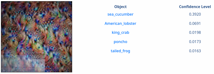recognize

Investigation

Let’s look at the activations, after feeding the image into the VGG19 network I have been using:

target = [model_vgg19.get_layer("block5_conv4").output]
model_vgg19_cutoff = tf.keras.Model(inputs=model_vgg19.input, outputs=target)
x = tf.keras.applications.vgg19.preprocess_input(np.expand_dims(img, axis=0))
activations = model_vgg19_cutoff.predict(x)
plt.plot(np.mean(np.mean(np.mean(activations, axis=0), axis=0), axis=0))

So the question we’re asking, is this the typical pattern for a dog or bison? Or maybe closer to the sea_cucumber pattern, in this 512-dimensional space?

Let’s have a look at the groenendael (1st image in Microscope) and sea_cucumber classes, as well as a few randomly selected ones. I downloaded the imagenet data and used this list to find the right files. Hmm I don’t really see a pattern by eye here, nor a similarity to above / excitation in index 4. In hindsight this makes sense, we wouldn’t expect the category to be simply 1-hot encoded in activation space, because a) there is not enough room, and b) there are more layers following so I would rather think of some clusters in the high dimensional activation space. Let’s maybe look some summary statistic, like the absolute distance in this 512-dim vector space.

So I take the training images, feed them into the network and read of the activations of the 512 nodes in the layer we are looking at (averaged over the 14x14 locations). Then I compute the distance as absolute distance between the vectors, 512-dimenisonal L2 norm. The image below shows the distance between the optimized “sea_cucumber essence” image and the activations of sea_cucumber training data (green), groenendael (blue), and a mix of 10 random classes (100 random images each). The blue curve shows the average activation-distance between randomly selected images of different classes. The code for all the following plots can be found in code_distances.py.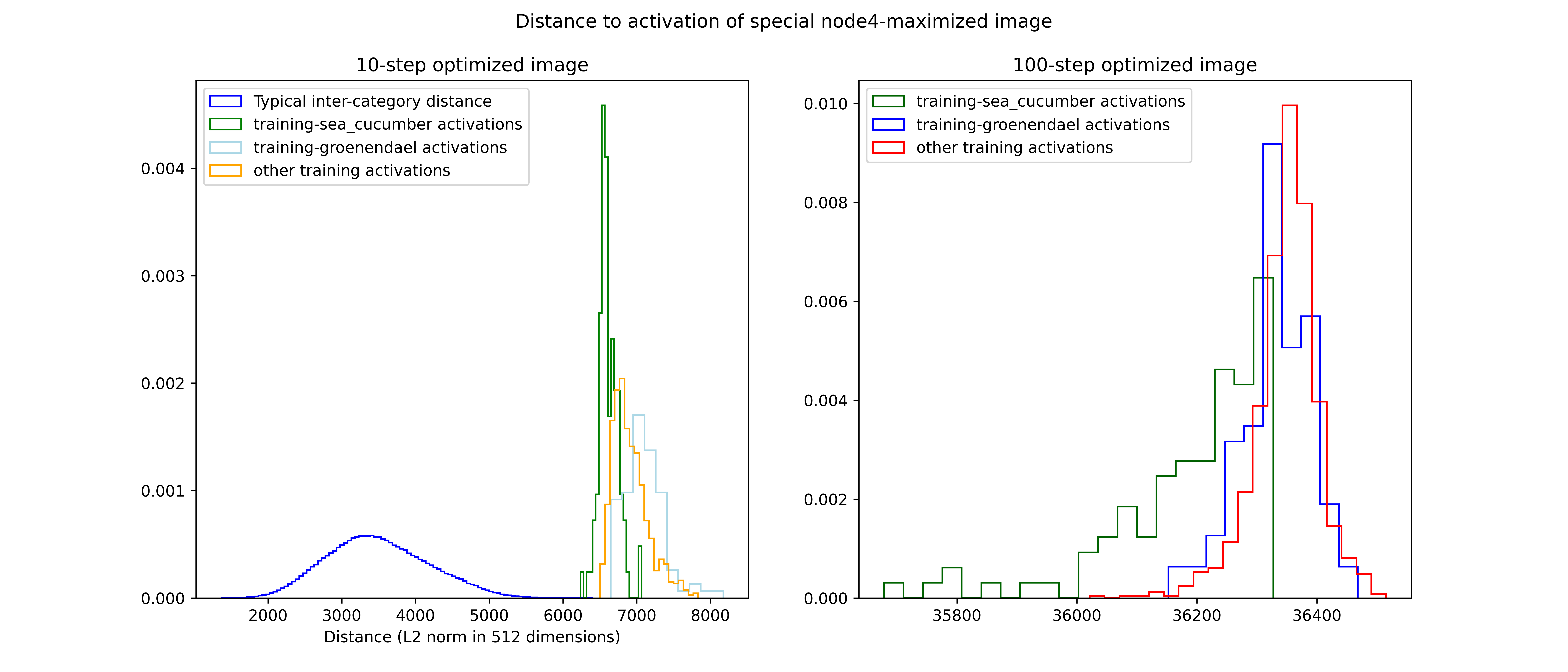

For context, here is the average distance between randomly selected images (grey), images from the same class (red) and images from different classes (blue): We learn three main things here:

Generally images of the same class seem to be nearer to each other in this 512-dim space than random / different classes, but the effect is not very strong. Of course we wouldn’t expect that the distance is the best measure of “closeness” between activations.
These numbers are all waaaay smaller than the ~7k and 36k we get from the “sea_cucumber essence” image. This tells us (somewhat unsurprisingly) that that optimized image is far outside the training distribution in at least this measure.
The sea_cucumber training data seems to give activations slightly closer to the “sea_cucumber essence” image – so maybe it’s just far outside the distribution but into the sea_cucumber direction?

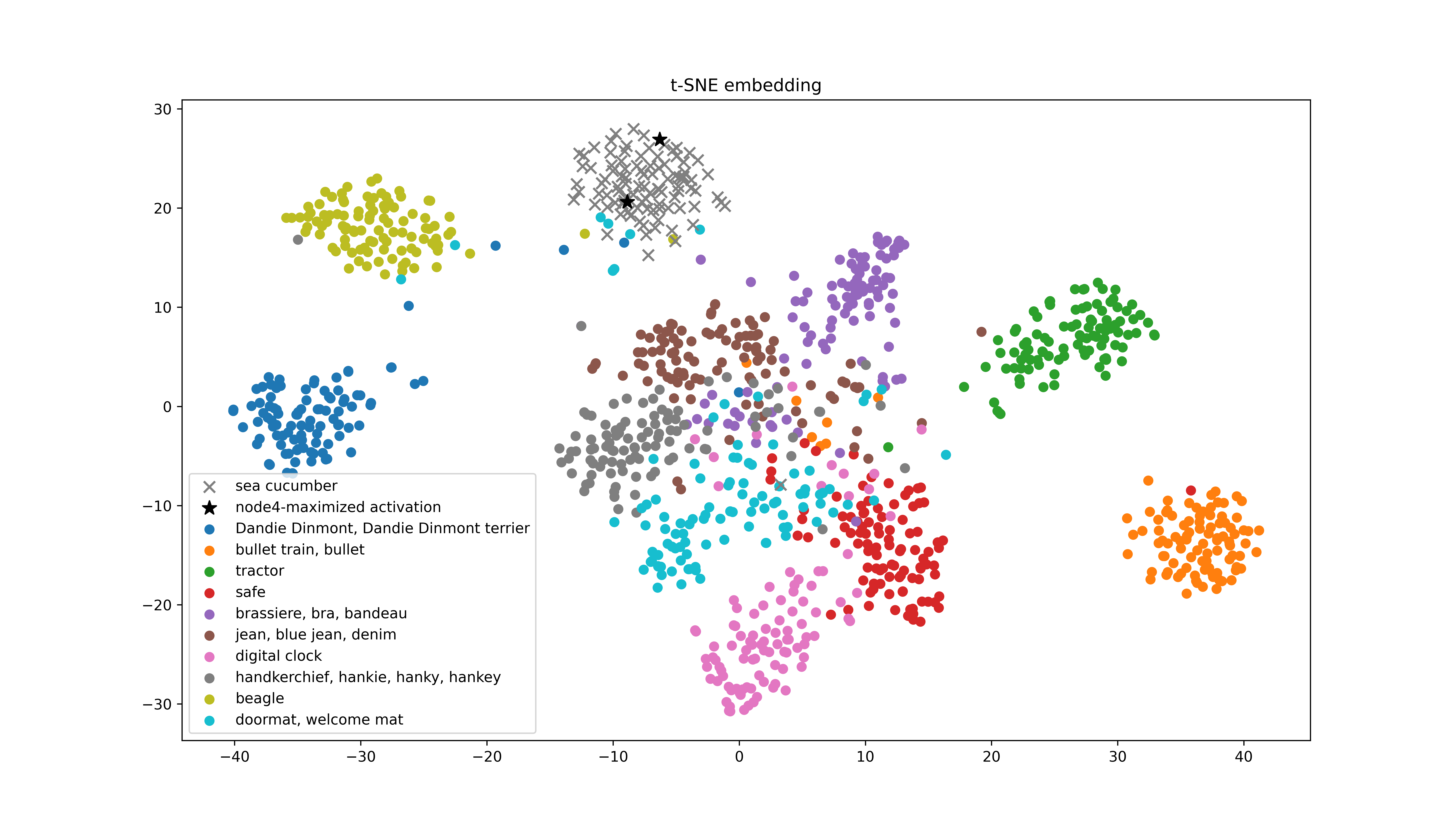
Naturally the L2-distance isn’t the ideal way to reduce the 512-d space into something plot-able. One method I found is t-SNE which projects the 512-dimensions into two parameters which we can plot: Looks like we get a nice separation (t-SNE does not know the labels) of different categories, and the “sea_cucumber essence” activations tend to lie within the sea_cucumber training data!

This doesn’t definitely answer the question, but I think it’s clear that this node4-maximized image ends up in a corner of parameter space which, even though it is “far away” (L2 distance), lies in a region that is clearly near the region that sea_cucumber training images lie in. Presented with this out-of-distribution image, and tasked with choosing between only the existing categories, the network decides for sea_cucumber.