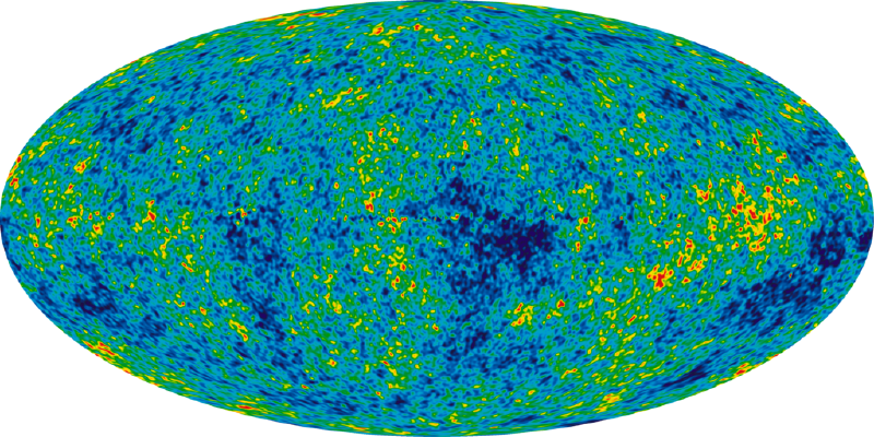
The Planck spacecraft is a satellite built to measure the Cosmic Microwave Background, the microwave radiation reaching us from the edge of the observable universe. Its goal is to detect tiny fluctuations (on the scale of 1 part in 100,000) of this radiation from different directions.
We use these observations to compare out theoretical models to reality. But because those fluctuations are based on randomness (quantum fluctuations in the early universe) we cannot predict the actual pattern on the sky. What we can predict, and test, are certain statistical properties. Most commonly we use the multipoles (usually referred to as the power spectrum) – what are those? They describe how correlated or different the radiation in directions looks, e.g. dipole relating to the correlation of opposite directions. Another way to think of this is the correlation of two directions at a certain (angular) distance. The dipole describes correlation of points 180 degrees apart, quadrupole 90 degrees etc. The 180th moment describes points separated by an angle of just 1 degree and this turns out to be the “strongest” correlation. In simple terms, we could say the circumstances in the early universe allowed matter and energy to travel such that spots about 40 million light years apart were very correlated.
For my work I frequently compute this power spectrum and compare it to the observations of Planck. For most of my work I used the code cobaya which automatically performs the calculation internally and returns the likelihood of a set of parameters being compatible with the Planck observations. One day I ran a model which was not included in cobaya, so I had to compute the likelihood myself and found surprisingly little documentation on the likelihood.
I did some reverse-engineeringreading of the cosmoslik wrapper to find out how it works, and want to write about the results here. But before I continue, if you just want to get the likelihood of a given power spectrum use cosmoslik’s cosmoslik.likelihoods module! Simply pass a dictionary of power spectra and you get the corresponding loglikelihood value.
Just out of curiosity though, I wanted to figure out how exactly I can use the Planck likelihoods without any external programs, also to make sure that the wrapper was still functioning. cosmoslik’s code turned out to be very helpful and largely what this is based on. So here’s my writeup of how to use the clik python code (this is still a wrapper for the C & Fortran code but since it comes together with the likelihood code from the Planck team I won’t dig deeper here). Firstly, assuming you have installed the likelihood and sourced the clik_profile script, you can import the clik python module and load a clik likelihood file:
from clik import clik
lowT = clik("/path/to/baseline/plc_3.0/low_l/commander/commander_dx12_v3_2_29.clik")
Now the function lowT can be called with a list as argument and returns the likelihood. To figure out which values to put in the list, we use the function lowT.get_lmax(). The former returns (29, -1, -1, -1, -1, -1) indicating it requires the TT spectra from l=0 to 29. The list maps to (TT, EE, BB, TE, ?, ?) where the latter two should be TB and EB but I’m not sure about the order. Next use lowT.get_extra_parameter_names() to get the nuisance parameters that need to be appended to the list, in this case ('A_planck',).
First let us get the power spectra, e.g. from CLASS
from classy import Class
cosmo = Class()
cosmo.set({'output': 'tCl pCl lCl', 'lensing': 'yes'})
cosmo.compute()
Cell = cosmo.lensed_cl()
Note that CLASS returns the power spectra in relative units while the likelihoods require absolute units (see Julien Lesgourgues’s comment here for some context), so we convert to uK² by multiplying by the mean CMB temperature squared.
Tcmb = 2.7255*1e6 #uK
Cl_TT = Cell['tt']*Tcmb**2
Also note that we just use the power spectrum C_ell, not the modified version D_ell. The latter is used as input for cosmoslik.
Finally we can call the likelihood with a list of spectra and nuisance parameters:
A_planck = 1.000442
lowT([*Cl_TT[:30], A_planck])
For something close to bestfit LCDM the result should be around -12.
For a more complex example, let’s look at the high-l TTTEEE likelihood. highTTTEEE.lmax shows us we need (2508, 2508, -1, 2508, -1, -1), i.e. the TT, EE and TE spectra, and in that order. highTTTEEE.extra_parameter_names lists a whopping 47 nuisance parameters which we have to pass in the right order as well. Tipp: You can get those in the right order from a dictionary wit something like nuisance_TTTEEE = [planck_nuisance_array[p] for p in highTTTEEE.extra_parameter_names]. Finally highTTTEEE(Cl_TT[:2509]+Cl_EE[:2509]+Cl_TE[:2509]+nuisance_TTTEEE) should return something like -1173, again for LCDM.
